Machine learning applied to showers in the OPERA
Abstract: in this post I explain how Machine Learning tools can be applied to particle physics. I'll discuss what is a particle shower, and when it appears in the OPERA and how clustering and classification techniques can help fundamental research.
This post is based on the research I've done for the OPERA experiment.
What are particle showers?
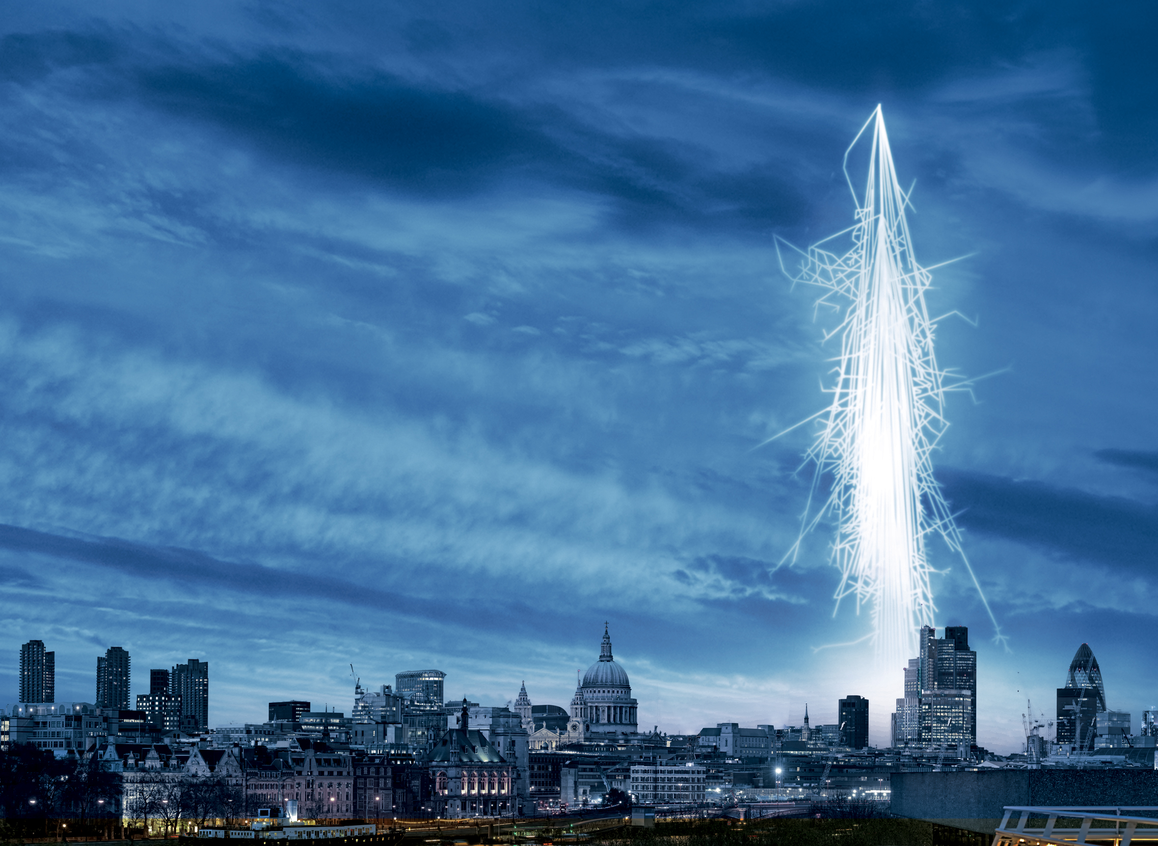
Illustration from University of Birmingham
When a charged particle (I'll consider an electron as an example) with extremely high energy passes through an atmosphere or material, it collides with atoms and produces new particles (converting its energy into mass of new particles). These newly-born particles also have high energy and also produce new particles when colliding with atoms, recursively forming a cascade of particles. Energy of an electron is enough for producing only finite number of new particles, thus this process stops and produced particles are stopped in the matter and absorbed.
There are atmospheric particle showers produced by high energy cosmic rays. But showers also can be observed in particle detectors, i.e. at the Large Hadron Collider, when a high-energy particle penetrates the detector.
What is OPERA?
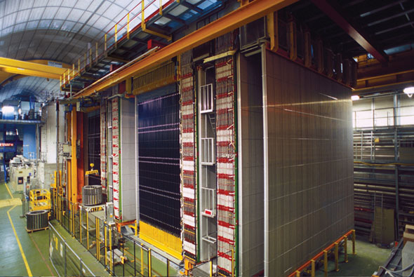
Inside OPERA,
image from symmetrymagazine.
The OPERA (Oscillation Project with Emulsion-tRacking Apparatus) is an international experiment in particle physics placed in Italy. Its main goal was to study the neutrino transitions (these studies performed by different experiments resulted in confirmation of neutrino oscillations and Nobel Prize 2015).
Neutrino can easily travel long distances through any matter (other known particles can't), so neutrino beam was sent through mountains from CERN (Geneva, Switzerland) to Gran Sasso (Italy).
OPERA has a huge detector, which contains around 150'000 bricks 8.5 kg each. Each brick contains interleaving layers of lead and nuclear emulsion. Nuclear emulsion (somehow resembles emulsion in old film photo cameras) keeps the tracks of particles for a long time (up to years), thus after scanning of emulsion we get a picture of the physics processes, whereas lead layers are needed to increase fraction of interacting neutrinos.
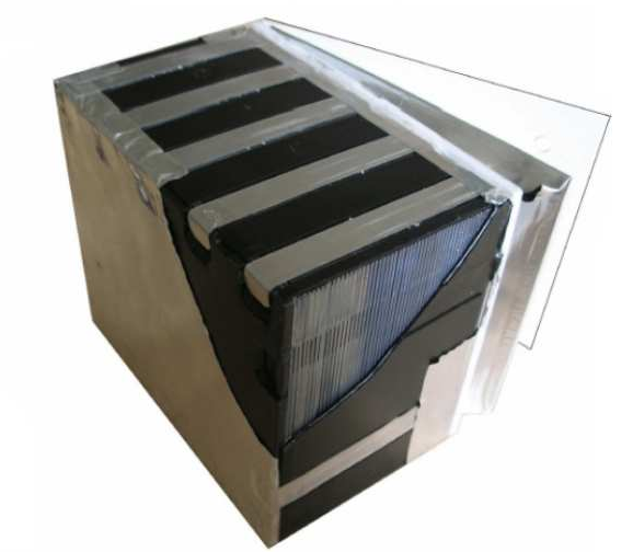
Opera brick, one of sides was removed to show layers of emulsion and lead, image source
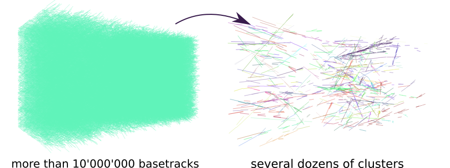
When emulsion is scanned, parts of the tracks are reconstructed (called basetracks), but the scanning is very precise (position resolution is few micrometers) and thus takes much time (complete scanning of a single brick takes days). The result of scanning is huge amount of basetracks (around $10^9$ basetracks in complete brick, or even more), however very few of these basetracks do correspond to some real particle track — most of the basetracks are noise, or instumental background as physicists say (bricks are collecting information for years before being extracted, developed and scanned, emulsion properties may become much worse, and during development fog grains appear, their random alignment is erroneusly recognized as a basetrack).
Cleaning the data with machine learning

Noise is absolutely dominating in the data (noise to signal ratio is around $10^4 - 10^6$), and to get something useful from this mess, serious cleaning of data is required. On the picture above you see visualization of scanning results, hardly any details are visible, but in fact this picture has only 1% of real amount of reconstructed tracks. And this is not the whole brick, but less than 1% of its complete volume. At such scales any analysis can be done only with programs.
There is not so much information that scanning provides: position of basetrack, it's direction and quality (typically in particle physics this information is provided with $\chi^2$ — quality of fit). The last one can reduce amount of background by several times, but we need something much more powerful.
The most important knowledge we have is that background doesn't have any geometrical structure, while signal basetracks are forming tracks or showers. Tracks are straight lines and have very simple geometrical pattern, but showers are more complicated.
Constructing good geometry-based features that grasp this difference is crucial. Good feature engineering coupled with appropriate machine learning algorithm gives very nice results as we will see.
Finding appropriate "neighboring" basetracks
To understand if this particular basetrack is a noise or corresponds to some real particle, we can look around and try to find appropriate "neighbours": if it is a track, then there should be basetracks left by the same particle on other layers, together they should form a straight line. If the basetrack is part of a shower, there should be basetracks left by a parent particle of by children particles (produced by current track).
Naive approach was to take position of the basetrack under consideration and to find closest basetracks in neighboring layers, but as shown on the scheme, this rarely selects appropriate basetrack. Our goal is to introduce such distance measure between basetracks, which takes into account:
- how close second basetrack to the direction line of the first one
- how close are directions of the basetracks
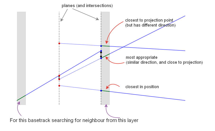
Simple and elegant solution is to introduce two planes and consider the intersection of planes and basetracks' direction lines. Basetracks lie on the same line if (and only if) intersection points coincide. And we can use sum of distances between projections as a distance between basetracks.
Sidenote: neighbours search is exetremely heavy if not optimized, for instance, computing distances between all pairs of basetracks takes $ O ( N^2_\text{basetracks} ) $, so some hacks are required to make it feasible.
Engineering geometrical features
After neighboring candidate basetracks are found, we need to estimate how likely selected basetracks are indeed part of some signal pattern (a track or a shower). The problem at hand is a binary classification problem (signal or noise), and can be approached with machine learning classification techniques. I used gradient boosting here and it provides very informative result, though insufficient to get the clear picture.

Features that help to disciminate signal and background are computed: angle between directions, impact parameters, mixed product of two directions and a vector connecting positions of basetracks, some projections, etc. Basetracks' $\chi^2$ qualities are also used. All of these features are combined into a single prediction by gradient boosting.
Looking further
To make the classification even stronger, we can collect more information about the neighbourhood. In particular, we can look at further layers (not only next or previous). Also we can make use of the information computed by gradient boosting at the previous step by providing it as a feature for new machine learning model (this trick is called stacking).

To understand whether some basetrack (red in this scheme) is part of the pattern or not,
we are analyzing basetracks (violet in this scheme) from different layers (preferring the tracks which have close direction and position).
For each of those tracks a set of features is computed,
and output of previous model for the nearest tracks from closest layers.
Analysis of the neighbourhood now has two stages and incorporates much more information about basetracks nearby. It is capable of reducing almost all the background at the price of losing around 50% of signal basetracks. That's how it looks like:
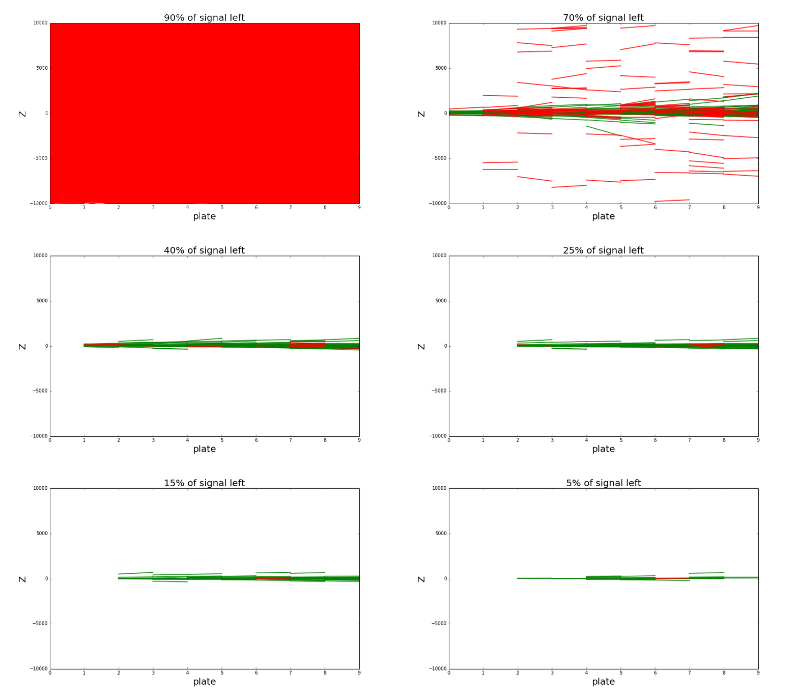 Looking at single particle shower when increasing classification threshold. Green tracks are part of a shower, background tracks (noise) are red.
Thresholding to keep around 50% signal tracks is enough to detect the presence of a shower quite easily.
There is also some minor background around the shower that's quite hard to get rid of,
but it doesn't cause any problems for shower detection.
Result so far
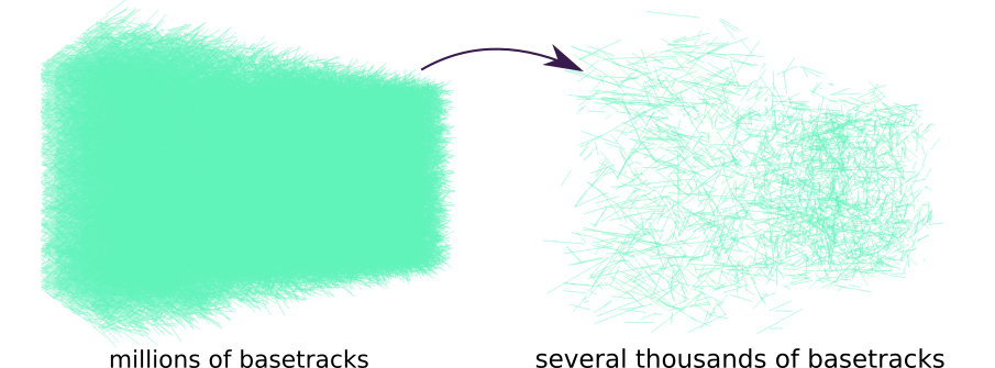
We reduced amount of tracks to analyze to some sensible amount, which is already great. Many patterns are already visible to a naked eye in 3d visualization (in particular, showers can be seen quite easily), but it would be much nicer if we could group basetracks into individual patterns.
Next time:
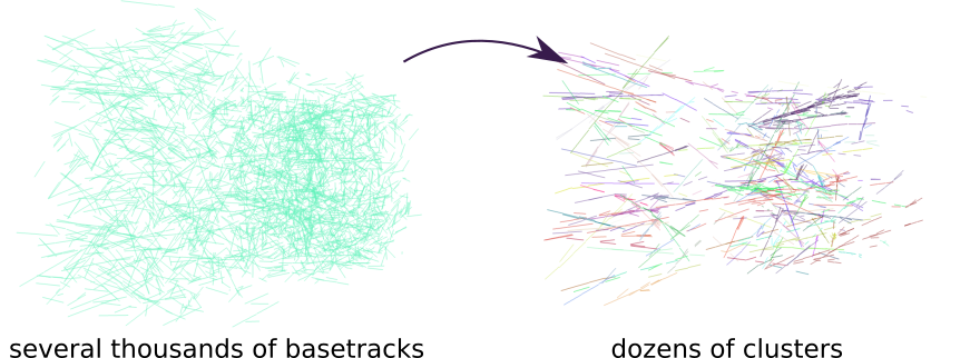
In the next post I discuss the clustering being applied to this problem.
 Gradient boosting
  Hamiltonian MC
  Gradient boosting
  Reconstructing pictures
  Neural Networks