Hamiltonian Monte Carlo explained

MCMC (Markov chain Monte Carlo) is a family of methods that are applied in computational physics and chemistry and also widely used in bayesian machine learning.

It is used to simulate physical systems with Gibbs canonical distribution: $$ p(\vx) \propto \exp\left( - \frac{U(\vx)}{T} \right) $$ Probability `$ p(\vx) $` of a system to be in the state `$ \vx $` depends on the energy of the state `$U(\vx)$` and temperature `$ T $`.

This distribution describes positions and velocities of particles in the gas, for instance. In bayesian machine learning, it defines distribution of model parameters (such as weights of a neural network).

Example: normal distribution is a Gibbs distribution

For example, consider a multivariate normal distribution: $$ p(\vx) \propto \exp\left( - \dfrac{1}{2} (\vx - \mu)^T \Sigma^{-1} (\vx - \mu) \right) $$ which corresponds to the following potential energy: $$ U(\vx) = \dfrac{1}{2} (\vx - \mu)^T \Sigma^{-1} (\vx - \mu), \qquad T=1. $$ Any distribution can be rewritten as Gibbs canonical distribution, but for many problems such energy-based distributions appear very naturally.

What is Monte Carlo (and why is it needed)?

Suppose that you want to study the properties of some model with thousands of variables (for lattice models that's very few!). For instance, average energy: $$ < U > = \int U( \vx ) \, p( \vx ) d \vx $$ is an integral over distribution. Computing this integral isn't possible, even using numerical approximations (lattice over 1000 variables is incredibly large).

By sampling from `$ p(\vx) $` an empirical estimate can be obtained: $$ < U > = \dfrac{1}{N} \sum_{i=1}^{N} U( \vx_i ), \qquad \vx_i \sim p ( \cdot ) $$ This is the idea of Monte Carlo: to compute average energy / speed of molecules in the gas, take random molecules and average their energy / speed.

Integration with distribution pdf (left) is replaced with averaging over samples from distribution (blue points on the right).
Rightmost plot demonstrates true samples on the energy surface, thus we can see corresponding energy `$ U(\vx) $`.

In modern programming languages there are functions to sample from simple distributions: uniform, normal, Poisson... There is no simple procedure to sample from Gibbs distribution: it is times more complicated, but possible using Markov Chains.

That's our goal: learn to sample from the canonical distribution.

How temperature influences canonical distribution:

unnormalized pdf `$ p(\vx) = p(x_1, x_2)$`

Energy `$ U(\vx) = U(x_1, x_2)$`

Distribution

Show
true samples
from distribution

temperature T:

Play with a temperature
and look at different distributions!

As intuition says, system has higher probability of staying in the states with lower energies. As temperature goes down, imbalance becomes stronger. When `$T$` tends to zero, the system stays in the state(s) with the lowest energy.

— So, we minimize energy?

Not really. Minimal-energy state is very important, but it is wrong to think that system can exist only in this state. To get good estimates of the system properties, a representative sampling of possible states is required (blue points demonstrate the desired distribution).

Pro tip: for bayesian people using maximum a posteriori estimation is the same as taking state with the lowest energy, while sampling corresponds to using bayesian posterior distribution. The latter has its benefits (though it's not simple to obtain!).

Why sampling from Gibbs distribution is complex?

In Gibbs distribution probabilities `$ p(\vx) $` are unknown. One can compute `$ U(\vx )$`, `$ T $` is known, but there is also a normalization coefficient `$Z$` $$ p(\vx) = \frac{1}{Z} \exp \left( - \frac{U(\vx)}{T} \right) \qquad Z = \int \exp\left( -\frac{U(\vx)}{T} \right) d \vx, $$ which can't be computed (except simple situations like multivariate normal).

All we have is a following ratio of probabilities (which doesn't depend on `$Z$`) $$ \dfrac{p(\vx_1)}{p(\vx_2)} = \dfrac{ \exp\left( - \frac{U(\vx_1)}{T} \right) }{ \exp\left(- \frac{U(\vx_2)}{T} \right) } = \exp\left( \frac{U(\vx_2) - U(\vx_1)}{T} \right) $$ and Markov chains can sample from the distribution using only this ratio. Let's see how.

Metropolis-Hastings algorithm for MCMC

The simplest Markov Chain process that can sample from the distribution picks the neighbour of the current state and either accepts it or rejects depending on the change in energy:

Algorithm produces a chain of states: `$ \vx_1, \vx_2, ..., \vx_n $` (green points).
Each time a candidate from a neighbourhood of the last state is selected `$\vx_n' = \vx_n + noise $` (noise is usually taken to be gaussian with some spread `$\sigma$`).

With probability `$ p = \min \left[1, \exp\left( \frac{U(\vx_n) - U(\vx_n')}{T} \right) \right] $` system accepts new state (jumps to the new state): `$ \vx_{n+1} = \vx_n' $` and with probability `$ 1 - p $` new state is rejected: `$ \vx_{n+1} = \vx_n $`.

Note, when energy is lower in new state `$ U(\vx'_n) < U(\vx_n)$` it is always accepted: `$ p = 1 $`. This way we give preference to the states with lower energies, while not restricting the algorithm to always decrease the energy. The lower temperature, the lower probability to increase energy.

Why does Metropolis-Hastings work?

The most interesting part is why this trivial algorithm is able to correctly sample from Gibbs distribution?

First thing to check is that single step of Metropolis-Hastings preserves canonical distribution. Formally, if `$\vx_n \sim p(\cdot)$` is Gibbs-distributed, then on the next step `$\vx_{n+1} \sim p(\cdot)$` is also Gibbs-distributed.

When the space of parameters `$\vx$` is discrete, this condition is written as: $$ \forall \vx \quad p(\vx) = \sum_{\vx'} p(\vx') \; p(\vx' \to \vx), \qquad p(\vx) \sim e^{-U(\vx) / T}, \; p(\vx') \sim e^{-U(\vx') / T} $$ with `$p(\vx' \to \vx)$` being probability of jumping from the state `$ \vx_n = \vx'$` to the state `$ \vx_{n+1} = \vx $`.

However, there is a much stronger condition, which guarantees preservation of canonical distribution. Namely, the detailed balance condition: $$ \forall \vx, \vx' \quad p(\vx') \; p(\vx' \to \vx) = p(\vx) \; p(\vx \to \vx') $$ implies previous condition (check it!). Markov chains with this condition are called reversible.

Reversibility is much easier to check. Below check is done for a Metropolis-Hastings step: $$ \frac{ p(\vx' \to \vx) }{ p(\vx \to \vx') } = \frac{ p(noise = \vx - \vx') \, p_\text{accept} (\vx' \to \vx) }{ p(noise = \vx' - \vx) \, p_\text{accept} (\vx \to \vx') } = $$ $$ = \frac{ p_\text{accept} (\vx' \to \vx) }{ p_\text{accept} (\vx \to \vx') } = \frac{ \min(1, e^{ (U(\vx') - U(\vx) ) / T }) } { \min(1, e^{ (U(\vx) - U(\vx') ) / T } )} = e^{ (U(\vx') - U(\vx) ) / T } = \frac{ p(\vx) }{ p(\vx') } $$ Due to this equality the MH sampling can converge only to canonical distribution, not something else.

Problems of Metropolis-Hastings algorithm

MH is very simple and quite general. The only thing required by algorithm is ability to compute energy `$U(\vx)$`. At the same time

too large step size `$ \sigma $` leads to a large fraction of rejected samples, while too small `$ \sigma $` makes very small steps, thus it takes long time to 'explore the distribution' (check this in demonstration!)
in high-dimensional spaces (very important use-case), MH explores the space very inefficiently because of it's random-walk behavior.
Guessing good direction in 1000 dimensions is incomparably harder than doing this for 2 dimensions!
MH can't travel long distances (significantly larger than `$ \sigma $`) between isolated local minimums

Sampling high-dimensional distributions with MH becomes very inefficient in practice. A more efficient scheme is called Hamiltonian Monte Carlo (HMC).

Hamiltonian Monte Carlo

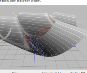
Physical analogy to Hamiltonian MC: imagine a hockey pluck sliding over a surface without friction, being stopped at some point in time and then kicked again in a random direction.

Hamiltonian MC employs the trick developed by nature (and well-known in statistical physics). Velocity `$v$` is added to the parameters describing the system. Energy of the system consists of potential and kinetic parts: $$ E(\vx, \vv) = U(\vx) + K(\vv), \qquad K(\vv) = \sum_i \dfrac{m \, v^2_i}{2} $$ Thus, velocities `$ \vv $` and positions `$ \vx $` have independent canonical distributions: $$ p(\vx, \vv) \propto \exp\left( \frac{-E(\vx, \vv)}{T} \right) = \exp\left( \frac{-U(\vx)}{T} \right) \, \exp \left( \frac{-K(\vv)}{T} \right) \propto p(\vx) \; p(\vv). $$ So once we can sample from joint distribution `$p(\vx, \vv)$`, we also can sample `$\vx$` by ignoring computed velocities `$\vv$`.

— How can we perform joint sampling?

– Just run physics simulation and get canonical distribution?

Very close: after you initialize the system parameters `$\vx, \vv$` and let it evolve ('slide') using physics equations $$ \dot{x}_i = v_i, \qquad m \dot{v_i} = - \dfrac{ \partial U (\vx)}{ \partial x_i } $$ during a long period of time, you'll not get a canonical distribution by collecting system states, because energy `$ E $` is conserved in the system. Physics allows only producing samples `$ (\vx, \vv) $` with the same energy `$ E(\vx, \vv) = E_0 $`, so we need to add something to 'plain physics' to get correct sampling.

For instance, gas molecules are colliding, what changes their velocity and energy in an unpredictable way. Similar idea can be used here, however there is a much simpler method – at some points in time velocity is resampled from `$p(\vv)$`, thus changing the total energy (this is how 'hit the puck in random direction' step appears).

Sampling from `$p(\vv)$` is very simple, because `$\vv$` is normally distributed.

— Is everything that simple?

Hit the puck, wait, stop it and then hit again.
This recipe sounds too simple to work, but if puck's trajectory could be computed precisely, it would be the solution.

However, the computer simulation is imprecise and this influences the result distribution. For instance, the energy isn't conserved in the simulation.

To minimize this influence, we can employ two tricks:

leapfrog numerical integration, which is reversible in time.
Reversibility makes it drastically easier to ensure detailed balance
Metropolis-Hastings rejections to compensate difference in energy between energy at the start and in the end. This way (quite few) rejected samples appear in HMC.

Pros and cons of Hamiltonian Monte Carlo

There is no free lunch, and Hamiltonian MC has its price: HMC uses not only energy `$U(\vx)$`, but also it's gradient. Hence possible applications are limited to the case when gradient exists and can be computed in reasonable time.

The major differences compared to Metropolis-Hastings are:

distances between successive generated points are typically large, so we need less iterations to get representative sampling
'price' of a single iteration is higher, but HMC is still significantly more efficient
Hamiltonian MC in most cases accepts new states (take a look at rejected samples in the demonstrations!)
still, HMC has problems with sampling from distributions with isolated local minimums
Investigate last distribution at low temperatures — 'puck' doesn't have enough energy to jump from the first minimum to the second over the energy barrier.

Bonus part: Passing energy barriers in Hamiltonian MC

As you probably noticed, that at low temperatures both MH and HMC can't overcome energy barrier (last distribution has two energy minima, separated by an energy barrier). Once system reaches some well-isolated local minimum, it gets stuck inside and probability to get to the different minimum becomes negligible, thus generated sample is 'incomplete'.

One empirical solution is manually restarting the generation from other start point, hoping to get stuck at the other minimum. Another way is to develop some algorithm to jump over energy barriers. One of such approaches is called tempering during a trajectory:

Play with tempering `$\alpha$` and trajectory length to get to the other minimum point!
Can you make it jumping between minimums frequently? What if you decrease temperature?

Idea behind tempering: the trajectory is split into two halves, which take equal time. During the first half, velocity is increased at each step by factor `$ \alpha $`: `$ \vv_\text{next} = \alpha \vv $`, during the second half velocity is decreased at each step by the same factor: `$ \vv_\text{next} = \frac{1}{\alpha} \vv $`.

This trick increases the energy of system during first half of trajectory and then decreases it.

While this process is reversible and can jump over energy barriers, the energies at the beginning and at the end are quite different. To correct this, rejection rule from Metropolis-Hastings algorithm is employed. Rejections become very frequent at low temperatures, thus amount of 'useless' computations becomes significant.

One needs to (blindly!) guess both 'slide time' and `$\alpha$`. An algorithm is quite sensible to both, in some cases producing too many rejections, in the other exploring the space inefficiently.
All in all: exploration is hard.