Machine learning in COMET experiment (part II)

In previous post I've written a short explanation of COMET - Japanese experiment in particle physics. This second post will be devoted to machine learning approach we developed for tracking (currently this is uses the information which is probably unavailable in online, but I still hope we will be able to get some online information and thus apply part of the approach as high-level trigger).

Local wire features

Anyway, the data we are going to use in classification is:

energy deposit for each wire
time of deposit for each wire

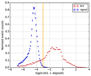
Let's look at their distributions:

Energy deposited on each 'wire' by signal and background tracks

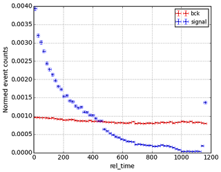Time elapsed starting from the moment of triggering till the time when particles are detected.

How do we obtain these values?

COMET uses straw chambers (which we call wires for simplicity), these are long tubes, which fill detector. They are filled with gas, which is ionized by moving charged particles (mostly, electrons).

After ionization, electrons and ions are moving to opposite directions, so we probably can estimate the moment of ionization by drift time (which is of course much greater compared to time of particle flight in detector). Drift time also gives approximate information about the distance between center of wire and track.

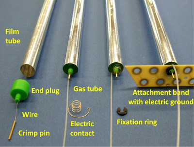Straw tubes used in many detector systems

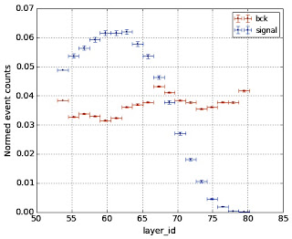
Finally, each wire has one more characteristic, namely, the distance to target:

Signal hits are more frequent on the inner layers by construction of experiment.

The time is counted from the moment of when trigger worked (it's another subdetector system). The event is 'recorded' starting from that moment.

The basic algorithm that was proposed (baseline algorithm) is using the cut on energy deposition. As you can see, there is really significant difference: energy deposited by background hits is higher. The reason is that background particles are moving slower, so they ionize more particles.

ROC AUC when we use the only feature - energy, is around 0.95, which seems to be very high. Nevertheless, it's not enough, since we have around 4400 wires, of which around 1000 gets activated (this number is called occupancy) within each measurement (event), while the signal track usually contains around 80 points.

So the event is represented using 4400 pairs (energy, time), of which most are zeros.

So the noise which passes through such basic filter is still very significant and there is large room for improvements.

First, let's combine all the information we have about the single wire (distance from center, time and energy deposition), let's call them wire features:

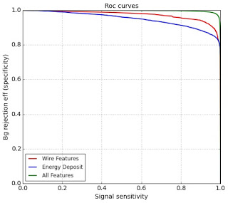ROC curves (using physical notation here), we see that usage of wire features made us able to twice decrease the background efficiency.

Neighbors features

Let me remind you, how the whole picture of hits in COMET detector looks like (we use here projection on the plane, orthogonal to beam line):

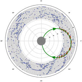Blue dots designate background hits, most of which are tracks of different charged particles, say protons; but some of them are simply noise.
Signal hits, which we are looking for, are red points forming an arc of circle. It's approximate radius is known ahead.

Simple but useful observation one can see in this plot: signal hits nearly always come together.
This implies that we can try using features collected from neighbours of point.

This drives to dramatic improvement of classification: we almost get rid of random noise tracks, still there are some coupled misidentified tracks. AUC is about 0.995, fpr (background efficiency) decreased by 4-5 times. In principle it suffices to use only information from left and right wires from the same layer.

Ok, I believe that was simple. Is there still something we missed and that could be improved?
For sure, this is the whole shape of the track. It’s time to try using this information.

Hough transform and circle shape

Hough transform was initially developed to detect lines and circles. Being quite trivial, it is one of the most effective algorithms in high energy physics.

After using GBDT trained on wire features and features of its neighbours, we are getting quite clean picture with very few false positives. All we want is to detect and remove possible isolated ’islands’ with misidentified background hits.

This is done by very approximate reconstruction of track centers. Since we know approximate radius of track center, we can use the Hough transform with fixed radius. It looks like:

Visualization of Hough transform for circles with fixed radius. We are trying to reconstruct the center of track, going through red points. Assuming that we know the radius of fitted track, all possible centers are laying on the circle with center in red point.

We discretize the space of possible track centers and for each point we reconstruct how likely it is the center of track. It is done using sparse matrices and some normalization + regularization (because otherwise tracks with few or many points will have very low/high probabilities).

Once we computed Hough transform, we leave only those centers, where hough transform is high, applying some nonlinear transformation there and applying inverse hough + some filtering. This way we obtain for each wire the probability that it belongs to some signal track.

Finally, we collect all the information we get for each wire:

local features (energy deposition, timing, layer_id)
features collected from neighbors
result of inverse hough transform

And train GBDT on these features to obtain final classifier. It’s ROC AUC is 0.9993 (100 times less probability of misordering)

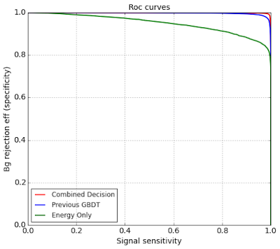Final classifier is red and it is very close to ideal one. The ROC AUC is about 0.9993

When we are comparing ROC curves at the threshold of interest (with very high signal sensitivity), things are bit worse, but still very impressing:

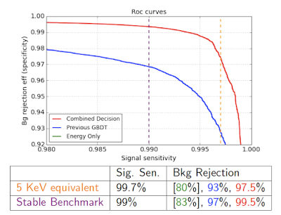At stable benchmark, the background yield decreased by factor of 34. Original ROC curve is not seen on the plot, since it is much lower.

Visualization of all steps

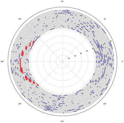Initial picture of hits in CyDET. Red are signal tracks, blue are background ones.

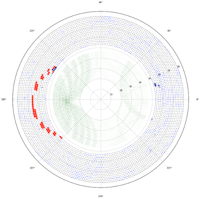After we apply initial GBDT (which uses wire features + neighbors), we have some bck hits (to the right, for instance). See the ’island’ of misidentified background to the right.
By greed dots we denote the possible centers of tracks. The bigger the point, the greater value of Hough transform image.

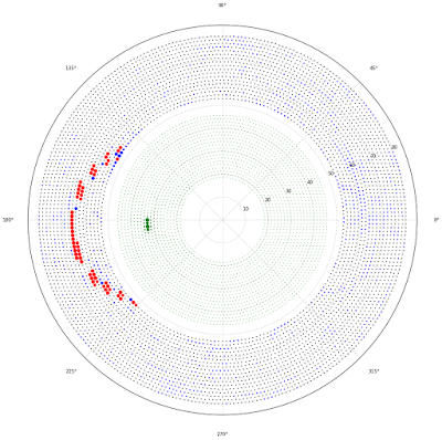Now we apply some non-linear transformations to leave only centers with very high probability. Then applying inverse hough transform and apply second GBDT, which incorporates also information from inverse Hough transform.

Conclusion

I’ve described how simple machine learning techniques coupled with well-known algorithms can produce a very good result, superior to many complex approaches.
These results are to be checked on better simulation data, when it will be ready. Also we have some ideas about possibilities of classification for online triggers, which use same ideas.